OpenCV-高斯金字塔

前言

机器视觉是本学期的专业课，上了几节课感觉和数字图像处理有很多知识点是相同的，毕竟机器视觉方面的研究底子都很厚，硬件软件方面都有涉及，实验一就是相机的几何标定，获得相机的内部参数什么的，虽然完成了，但事后总感觉有点意义不明，毕竟课堂上学到的东西一点没用到，以后也不需要这样测定几何参数。还在课堂上得知神经网络的小趣闻，那说实话，科学界普遍不看好神经网络也不是没有原因，这东西本质就是“映射”，但是没有什么理论基础，没人知道为什么会这样，出乎意料就是效果不错，在识别领域反超了传统计算机视觉。但是由于不清楚底层原理，整个模型出来了就不能再改，改了就得重新训练，创新基本就是几个构成部分增删重组，给人的感觉就是碰运气，时间成本相当高。相反的，机器视觉在基础研究领域有着深厚的根基，所以相对有迹可循。

本次实验是生成图像的高斯金字塔，本质也就是生成在不同远近程度下的缩略图。本实验运用到OpenCV、Matplotlib和numpy三个库，但不会直接调用OpenCV中的pyrDown函数，而是尽量从原理出发进行编程实现。

算法原理

高斯滤波

高斯滤波器是一种线性平滑卷积滤波器，通常用于图像处理中的平滑滤波操作。该滤波器将每个像素点周围的像素点按照权重进行平均，用以实现图像的平滑效果。

高斯滤波器的核心思想是对图像进行加权平均处理，在这个过程中使用高斯函数来确定权重值。高斯函数是一种常见的连续分布函数，其形式为:

其中，x表示距离中心像素的偏移量，σ表示高斯函数的标准差。应用高斯函数可以得到一个呈钟形的权重函数，并且越靠近中心点的权重越高，越远离中心点的权重越低。

在高斯滤波中，我们采用一个大小为n*n的滤波器核对图像进行卷积操作。核中的每项权重使用高斯函数计算而成，因此每个像素点都会受到周围像素点的影响。中心点的权重最大，越靠近中心点的像素的权重越高，而越靠远离中心点的像素的权重越低。通过这种方式，我们就能够非常有效地去除图像中的噪声、平滑图像等。

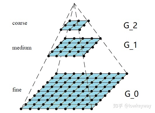
高斯图像金字塔

图像高斯金字塔是一种在图像处理中常用的方法，用于对图像进行多尺度分解和降采样。该方法通过对图像进行平滑和下采样操作，生成图像的不同分辨率的版本，从而实现多尺度图像处理。

生成过程为：

首先将原图像作为最底层图像 level0（高斯金字塔的第0层）
利用高斯核对其进行卷积
对卷积后的图像进行下采样（去除偶数行和列）得到上一层图像G1
将此图像作为输入，重复2与3的操作得到更上一层的图像，反复迭代多次
最后形成形成一个金字塔形的图像数据结构，即高斯金字塔。

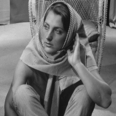
算法实现及结果分析

高斯滤波函数

本次实验我采用Python语言，素材为冈萨雷斯图片素材，为实验方便裁剪为正方体。

本实验运用到OpenCV、Matplotlib和numpy三个库。

1
2
3

import cv2
import numpy as np
import matplotlib.pyplot as plt

根据高斯滤波的原理编写：

def gaussian_blur(img, K_size=3, sigma=1.3):  
    """ 
    高斯滤波器 
    :param img: 输入图像 
    :param K_size: 核函数大小 
    :param sigma: σ 
    :return: 滤波后的图像 
    """  
    H, W, C = img.shape  
    # Zero padding  
    pad = K_size // 2  
    # 黑边填充后会出现大黑边  
    # out = np.pad(img, ((pad, pad), (pad, pad), (0, 0)),'constant', constant_values=0)  
    # 用图像边缘像素进行填充  
    out = cv2.copyMakeBorder(img, pad, pad, pad, pad, borderType=cv2.BORDER_REPLICATE)  
    # 创建和函数  
    K = np.zeros((K_size, K_size), dtype=float)  
    for x in range(-pad, -pad + K_size):  
        for y in range(-pad, -pad + K_size):  
            K[y + pad, x + pad] = np.exp(-(x ** 2 + y ** 2) / (2 * (sigma ** 2)))  
    K /= (2 * np.pi * sigma * sigma)  
    K /= K.sum()  
    tmp = out.copy()  
    # 滤波  
    for y in range(H):  
        for x in range(W):  
            for c in range(C):  
                out[pad + y, pad + x, c] = np.sum(K * tmp[y: y + K_size, x: x + K_size, c])  
    # 将数值转化为RGB限制范围  
    out = np.clip(out, 0, 255)  
    # 转化格式：unit8  
    out = out[pad: pad + H, pad: pad + W].astype("uint8")  
    return out

这边有一个注意点，在滤波之前的，为了减小边缘处像素对计算的影响，一般来说我们需要给图像填充边缘，边缘大小一般为(模板大小// 2)。这时候有两种方案填充方案。第一种方案是采用常数填充，第二种方案是直接采用图像边缘像素填充。我选择第二种方案，具体原因在[测试与结果分析](# 测试与结果分析)部分说明。

使用以下代码测试滤波效果：

# 高斯滤波 
GaussianBlur_imag1 = gaussian_blur(img, 3, 1)
GaussianBlur_imag2 = gaussian_blur(img, 5, 1)
GaussianBlur_imag3 = gaussian_blur(img, 5, 3)

title_list = ["Original", "size=(3,3)\n σ=1", "size=(5,5)\n σ=1", "size=(5,5)\n σ=3"]
img_list = [img, GaussianBlur_imag1, GaussianBlur_imag2, GaussianBlur_imag3]

# 展示图像 
plt.figure(dpi=100, figsize=(10, 10))
for i in range(1, 5):
    plt.subplot(2, 2, i)
    plt.title(title_list[i - 1])
    plt.imshow(img_list[i - 1])

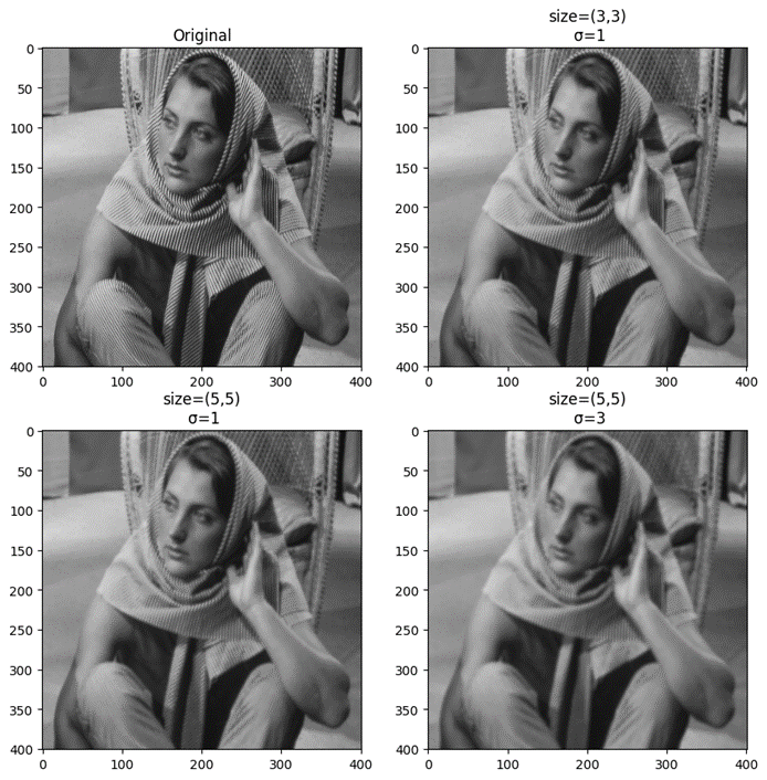
高斯滤波器滤波效果如下所示：

从结果可以看出，平滑效果随着kernel与σ的增大而增强。高斯滤波后有明显的模糊现象。

生成高斯金字塔

图像高斯金字塔有两个过程，一是向下采样，二是高斯滤波。

向下采样本质就是缩小图像尺寸来达到降低分辨率的目的，以生成图像的缩略图。缩小的过程可以采用OpenCV自带的resize函数来实现。

def downsample(img, scale=0.5):
    """ 
    下采样 
    :param img: 输入图像 
    :param scale: 缩放比例，默认为0.5 
    :return: 下采样后的图像 
    """
    h, w = img.shape[0:2]
    new_h = int(h * scale)
    new_w = int(w * scale)
    # 采用双线性的方法 
    result = cv2.resize(img, (new_h, new_w), interpolation=cv2.INTER_LINEAR)
    return result

在更改大小时，插值方式我采用了最常用且效果不错的双线性插值。默认按照缩放倍率0.5进行缩放。

在高斯滤波和下采样实现的基础上，可以按照原理实现高斯金字塔函数的编写。

def pyramid(imag, floors, guass_kernel):
    """ 
    生成图像高斯金字塔 
    :param imag: 输入图像 
    :param floors: 输入高斯金字塔层数 
    :param guass_kernel: 高斯滤波核大小 
    :return: None 
    """
    # 打印当前金字塔层数 
    print(f"Total Gaussian pyramid {floors} levels")

    if floors == 1:
        plt.figure(dpi=150, figsize=(8, 8))
        # 得到第零层 
        plt.title("Gaussian pyramid\n 0 level")
        plt.imshow(img)

    else:
        x, y = factor(floors)[0:]
        # 保持x>y 
        x, y = swap(x, y)
        # 打印布局大小 
        print(f"Sub-map layout: row-{x} column-{y}")
        # 绘制图像 
        plt.figure(dpi=150, figsize=(12, 8))
        plt.subplot(x, y, 1)
        # 得到第零层  
        plt.title("Gaussian pyramid\n 0 level")
        plt.imshow(img)
        for i in range(2, floors + 1):
            imag = downsample(imag)
            imag = gaussian_blur(imag, K_size=guass_kernel, sigma=1.3)
            plt.subplot(x, y, i)
            plt.title(f"Gaussian pyramid\n {i - 1} level")
            plt.imshow(imag)
        # 设置子图间的水平和垂直间距 
        plt.subplots_adjust(wspace=0.5, hspace=0.35)
    plt.show()
    print("Image created successfully")

由原图像作为高斯金字塔的第0层，之后的层数按照采样和滤波的过程循环进行。需要注意的是，因为下采样是按照0.5倍率进行缩放，为了避免报错，因此输入图像最好为正方形尺寸。在代码第22行出现了一个名为factor()的函数，下面我们会讲到这个函数的作用。

输出图像排布设置

为了更好展示每次缩放后的图像细节，我采用matplotlib对图像进行展示。但是根据使用者每次输入的floors的不同，所生成的子图数量是不一样的。举几个例子：

输入5时，排布可以为subplot(1,5,i)或者subplot(5,1,i)
输入8时，排布可以为subplot(2,4,i)或者subplot(4,2,i)
输入6时，排布可以为subplot(6,1,i)、subplot(1,6,i)、subplot(2,3,i)、subplot(3,2,i)

输出图的数量总是随着输入在改变，这时候就需要考虑如何排布。

最为简单的思路就是进行因式分解，而且需要保证行数大于列数，这样输出的图像更加美观。按照分析编写出以下函数。

# 获得子图的排布
def factor(num):
    """
    根据获得子图排布
    :param num: 金字塔层数
    :return: 子图排布
    """
    list1 = []
    for i in range(2, 10):
        temp = int(num / i)
        if (temp >= 1) & (temp * i == num):
            list1.append(i)
            list1.append(temp)
            break
    # list1.append(1) if len(list1) == 1 else None
    return list1

输入示例：

输入6：[2,3]
输入5：[5,1]

假设输出结果为[a,b]，那么根据示例1，很可能会出现a<b的情况，这样就会出现行数大于列数，这样排布是不美观的，所以我们需要在设当场合将他们交换，使之在任何情况都保持a>b。

1 2	# 交换 def swap(a, b): return (b, a) if a > b else (a, b)

测试与结果分析

测试代码：

if __name__ == '__main__':
    img = cv2.imread("./input/test.png")
    floors = int(input("Please enter the floors of the pyramid\n（The input number is between 1 and 8）："))
    if (floors < 1) | (floors > 8):
        print("The floors must be between 1 and 8 ")
        exit()
    pyramid(img, floors=floors, guass_kernel=5)

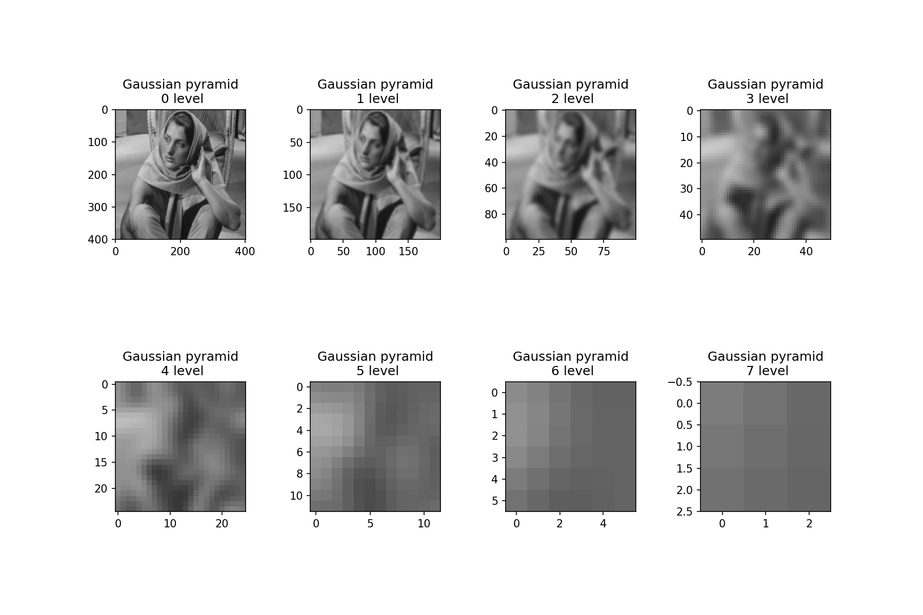
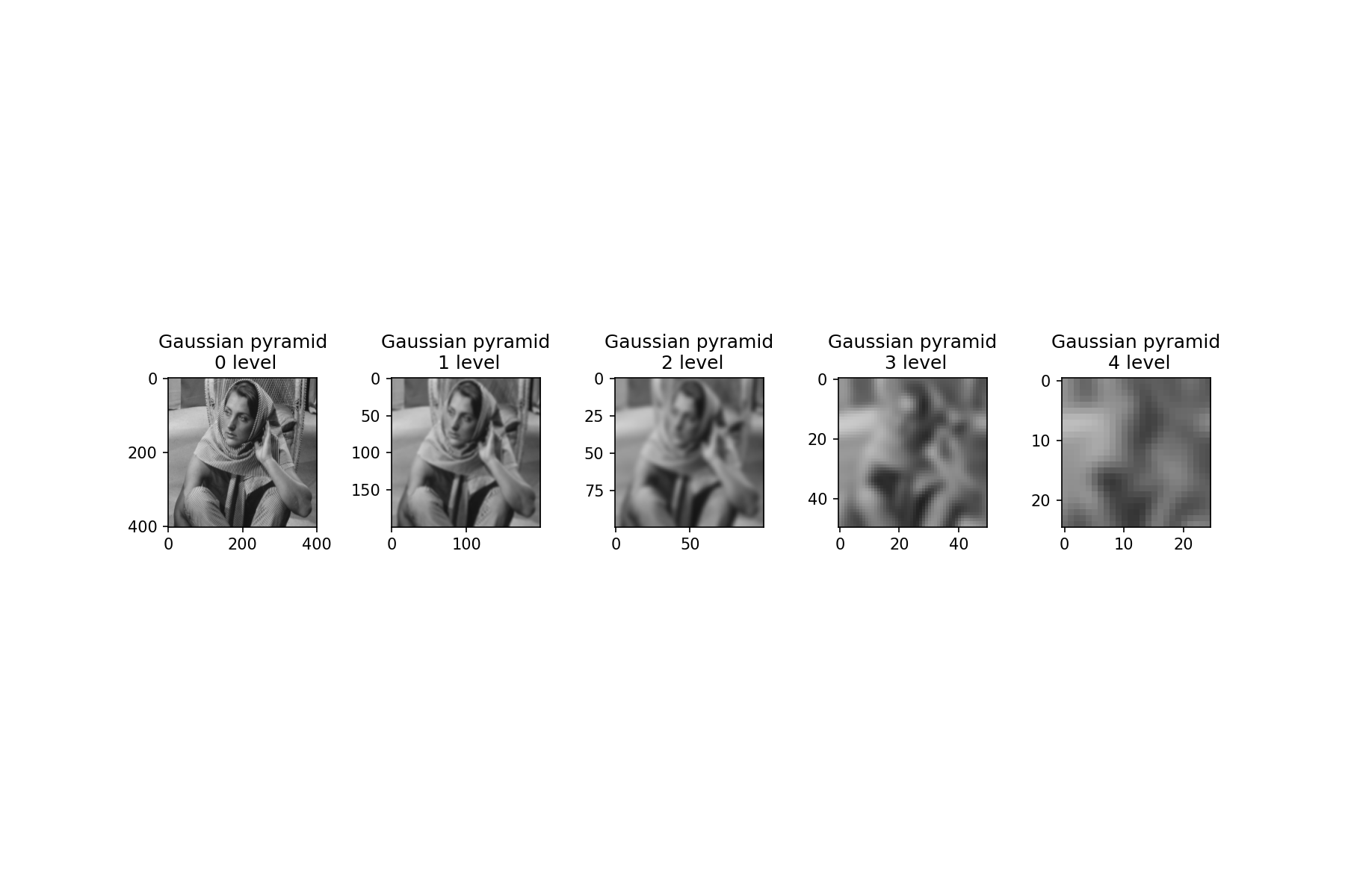
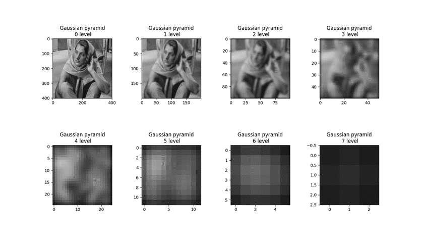
当floors=8时，得到的图像高斯金字塔每层图像和输出结果如下：

当floors=5时，图像与输出结果如下：

可以看到生成的结果没有出现很大的差错，排布的结果也是比较美观的，当然不好的地方就是能看到非常明显的白边，这是由于figsize的限定大小所决定的，因为figsize无法根据floors的变换自适应图像(典型的就是标题重叠)，尝试使用subplots_adjust调整子图间距也不是很好，迫不得已使用了figsize=(12,8)的大小设定。

有一个注意点，在高斯滤波时，有两种填充方案。

第一种：直接用常数0进行填充。
第二种：拿图像的边缘像素进行填充。

如果采用第一种方案进行填充，可以达到平滑图像边缘像素的目的，但是在生成高斯金字塔这个需要多次平滑的过程中，很容易出现图像黑边的情况，直接影响了高斯金字塔的生成效果，因此不能使用这种方案。

展示一下用第一种方案的floors=8的输出结果：

可以看到黑白的影响随着金字塔层数的增加是逐渐加剧的,第7层甚至出现完全黑图的情况，这严重影响了生成的结果。因此最终我选择第二种填充方案。

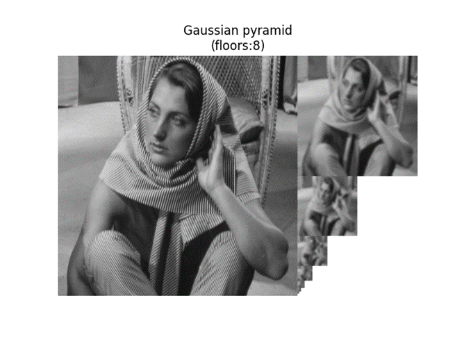
金字塔效果

因为老师想要我们观察图像的细节变化，所以我采用了Matplotlib一张一张拼接展示，为了美观，自己也按照老师课件上的金字塔效果编写了一个程序，总体的处理流程还是一样，只是多了拼接图像的过程，这次就直接使用pyrDown进行实现。

import cv2
import numpy as np
import matplotlib.pyplot as plt

# 读取图像
img = cv2.imread("./input/test.png")
img = cv2.cvtColor(img, cv2.COLOR_BGR2RGB)
print(f"Original: width-{img.shape[0]} height-{img.shape[1]}")


def Extended_Image(img1, img2, model=1):
    if model == 1:
        if img1.shape[1] < img2.shape[1]:
            temp = img1.copy()
            img1 = img2.copy()
            img2 = temp

        add_height = img1.shape[0] - img2.shape[0]
        add_img = np.zeros((add_height, img2.shape[1], 3), np.uint8) + 255
        result = np.vstack((img2, add_img))

    elif model == 2:
        if img1.shape[0] < img2.shape[0]:
            temp = img1.copy()
            img1 = img2.copy()
            img2 = temp
        add_width = img1.shape[1] - img2.shape[1]
        add_img = np.zeros((img2.shape[0], add_width, 3), np.uint8) + 255
        result = np.hstack((img2, add_img))
    return result


# 下采样
def downsample(img, scale=2):
    h, w = img.shape[0:2]
    new_h = int(h / scale)
    new_w = int(w / scale)
    result = cv2.resize(img, (new_h, new_w), interpolation=cv2.INTER_LINEAR)
    return result


def init_guass(img, kernel=(3, 3)):
    return cv2.GaussianBlur(img, kernel, 1.5)


floors = int(float(input("Please enter the floors of the pyramid：")))

if floors == 1:
    print(f"当前输出的金字塔的层数为：{floors}")
    result = init_guass(img, kernel=(5, 5))

elif floors < 1:
    print("floors只能为大于0的整数")

elif floors > 1:
    print(f"Total Gaussian pyramid {floors} levels")
    img_1 = cv2.pyrDown(img)
    result = init_guass(img_1, kernel=(5, 5))
    img_1 = result.copy()
    for i in range(floors - 1):
        img_2 = downsample(img_1)
        img_2 = init_guass(img_2, kernel=(5, 5))
        temp_img = Extended_Image(img1=result, img2=img_2, model=2)
        result = np.vstack((result, temp_img))
        img_1 = img_2.copy()

    temp_img = Extended_Image(img1=img, img2=result, model=1)
    result = np.hstack((img, temp_img))

plt.figure(dpi=150)
plt.title(f"Gaussian pyramid\n(floors:{floors})")
plt.axis("off")
plt.imshow(result)
plt.show()

当输入floors=8时，输出结果如下：